Comparisons with BGEP ULS sea ice draft estimates

Comparisons with BGEP ULS sea ice draft estimates#

Summary: In this notebook, we produce comparisons of the gridded ICESat-2 sea ice thickness data with draft measurements obtained from Upward Looking Sonar moorings deployed in the Beaufort Sea.

Raw data link: https://www2.whoi.edu/site/beaufortgyre/data/mooring-data/2018-2021-mooring-data-from-the-bgep-project/

Notes:

With more years of data we hope to explore seasonal de-trending of the data. Current tools (e..g seasonal_decompose from statsmodel) require more years of data then currently provided by the ICESat2-/BGEP overlap period (2018 to 2021)
Some previous studies have removed zero draft values from ULS before undertaking these comparisons. Hard to know what is best here. ATL10 are available for passive microwave concentrations > 50%. Our gridded thickness data includes all this (baring some additional anomaly filters) so could also include reasonably large stretches of thin ice/open water too. I have toyed with included a ‘thickness where we have ice’ variable too, which I could easily include later, then we would just compare this to positive values of ULS draft?
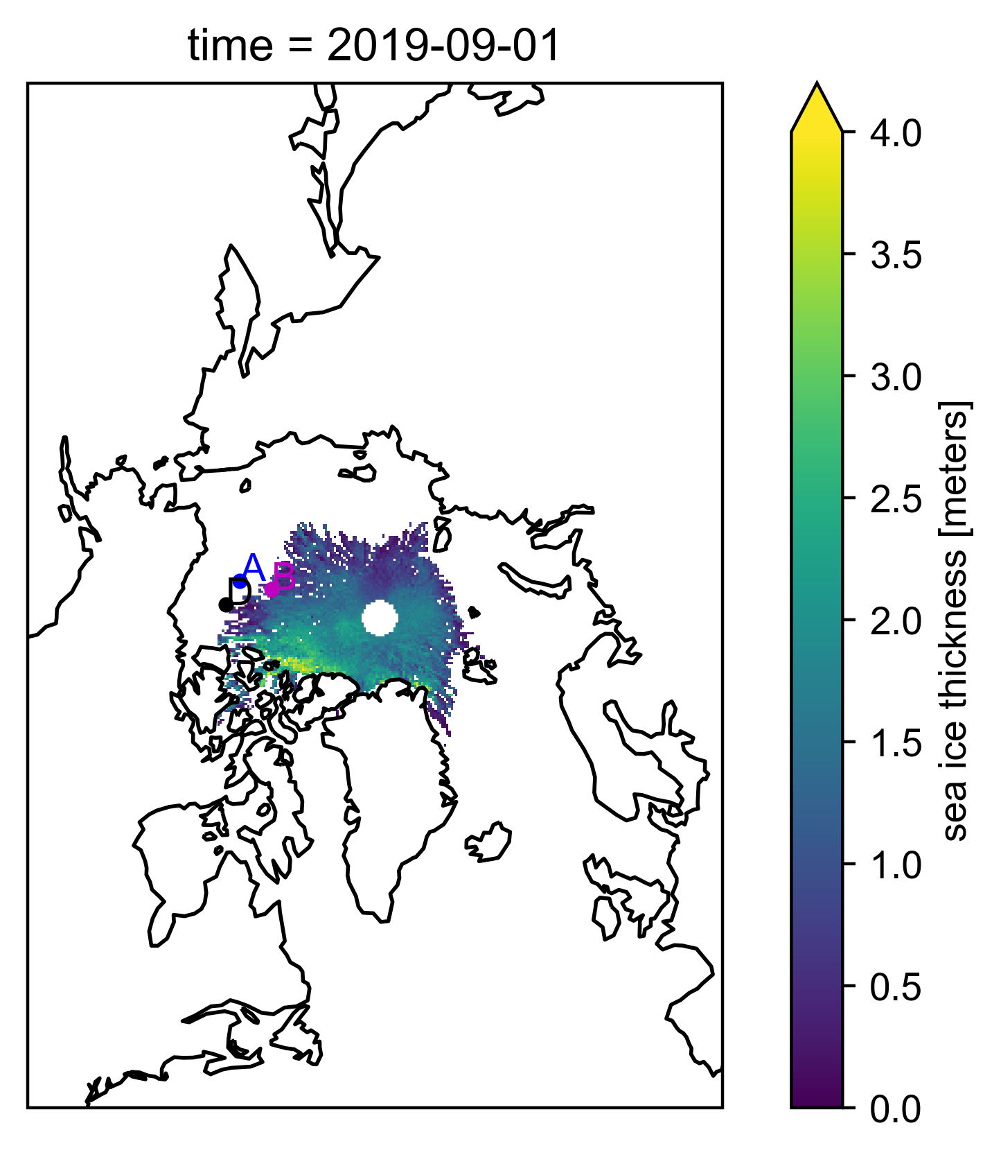
Could require a minimum number of IS2 grid-cells, but would perhaps need to depend on the chosen comp_res. Note how in some September/October months there appears to be no data overlap, I included some maps at the end to highlight this more, the moorings are right on the edge of the ice pack in September 2019 for instance.
We do a fair bit of averaging to try and reduce noise from various sources, including sampling differences/representation errors. One more direct way of dealing with this would be to use the day_of_the_month information in the IS-2 thickness data to see what actual day the nearest grid-cells to the moorings best represent and comapre that to the daily ULS data. This leads to using the along-track data too, hard to know when to stop..
We could have made better use of Pandas in this analysis but I was a bit time pressured.

Version history: Version 1 (01/01/2022)

Import notebook dependencies#

import xarray as xr 
import pandas as pd
import numpy as np
import itertools
import pyproj 
from netCDF4 import Dataset
import scipy.interpolate 
from utils.read_data_utils import read_book_data # Helper function for reading the data from the bucket
from utils.plotting_utils import compute_gridcell_winter_means, interactiveArcticMaps, interactive_winter_mean_maps, interactive_winter_comparison_lineplot # Plotting
from scipy import stats
import datetime
# Plotting dependencies
import cartopy.crs as ccrs
from textwrap import wrap
import hvplot.pandas
import holoviews as hv
import matplotlib.pyplot as plt
from matplotlib.axes import Axes
from cartopy.mpl.geoaxes import GeoAxes
GeoAxes._pcolormesh_patched = Axes.pcolormesh # Helps avoid some weird issues with the polar projection 
%config InlineBackend.figure_format = 'retina'
import matplotlib as mpl

mpl.rcParams['figure.dpi'] = 200 # Sets figure size in the notebook

# Remove warnings to improve display
import warnings 
warnings.filterwarnings('ignore') 

# Read/download the IS-2 thickness data 
# NG: don't need the CryoSat-2 data here but could if you want to explore those comparisons too...
book_ds = read_book_data()

# Issue in how region mask was assigned
book_ds['region_mask'] = book_ds['region_mask'].isel(time=0, drop=True)

# Estimate ice draft from the ICESat-2 data for more direct comparison with ULS draft measurements
# NB: Another option (not taken) is to simply multiply ULS drafts by 1.1 to convert to thickness (AWI do this)
# Include extra var = '_int' to use interpolated values, not recommended for validation purposes. 
int_str=''
book_ds['ice_draft'] = book_ds['ice_thickness'+int_str] - book_ds['freeboard'+int_str]+ book_ds['snow_depth'+int_str]

# Initialize map projection and project data to it

out_proj = 'EPSG:3411'
out_lons = book_ds.longitude.values
out_lats = book_ds.latitude.values

mapProj = pyproj.Proj("+init=" + out_proj)
xptsIS2, yptsIS2 = mapProj(out_lons, out_lats)

start_date = "Nov 2018"
end_date = "Apr 2021"
IS2_date_range = pd.date_range(start=start_date, end=end_date, freq='MS') # MS indicates a time frequency of start of the month
IS2_date_range = IS2_date_range[((IS2_date_range.month <5) | (IS2_date_range.month > 8))]
IS2_date_range_strs=[str(date.year)+'-%02d'%(date.month) for date in IS2_date_range]

# This is the value in meters of the aggreation length-scale for the ICESat-2 data
comp_res=25000

# Wrange ULS data
# Could really convert this to another data wrangling notebook and store the derived output as netcdfs

dataPathULS='./data/'

def get_ULS_dates(uls_mean_monthly_draft, uls_dates, date):
    #print(date)
    a = uls_mean_monthly_draft[uls_dates==date].values[0]
    return a

def get_uls(letter):
    if letter=='a':
        print('Mooring A (75.0 N, 150 W)')
        uls_x, uls_y = mapProj(-150., 75.)
    if letter=='b':
        print('Mooring B (78.4 N, 150.0 W)')
        uls_x, uls_y = mapProj(-150., 78.4)
    if letter=='d':
        print('Mooring D (74.0 N, 140.0 W)')
        uls_x, uls_y = mapProj(-140., 74.)
 
    uls = pd.read_csv(dataPathULS+'uls18'+letter+'_draft.dat', sep='\s+',names = ['date', 'time', 'draft'], header=2)
    utc_datetime_uls = pd.to_datetime(uls['date'], format='%Y%m%d')
    uls_mean_daily_draft = uls['draft'].groupby([utc_datetime_uls.dt.date]).mean() 

    uls_mean_monthly_draft = uls['draft'].groupby([utc_datetime_uls.dt.to_period('m')]).mean() 
    #print(uls_mean_monthly_draft)
    
    return uls_mean_daily_draft, uls_mean_monthly_draft, uls_x, uls_y

uls_mean_daily_draft_a, uls_mean_monthly_draft_a, uls_x_a, uls_y_a = get_uls('a')
uls_mean_daily_draft_b, uls_mean_monthly_draft_b, uls_x_b, uls_y_b = get_uls('b')
uls_mean_daily_draft_d, uls_mean_monthly_draft_d, uls_x_d, uls_y_d = get_uls('d')

Mooring A (75.0 N, 150 W)

Mooring B (78.4 N, 150.0 W)

Mooring D (74.0 N, 140.0 W)

def grid_IS2_nearby(date, uls_x, uls_y, res=75000):
    #print(date)
    IS2 = book_ds.ice_draft.sel(time=date)
    xptsIS2=IS2.xgrid.values
    yptsIS2=IS2.ygrid.values
    #dist = np.sqrt( (xptsIS2 - uls_x)**2 + (yptsIS2 - uls_y)**2 )
    
    #IS2_uls = IS2.where(dist<res).mean()
    
    #print('Number of valid IS-2 grid cells in month '+str(date)[0:7]+':', np.count_nonzero(~np.isnan(IS2.where(dist<res))))
    
    #Another option I first explored, coarsen the data then do nearest neighbor...provided similar results but above is more flexible.
    #if coarse_res>1:
    #Coarsen array by coarse_res in x/y directions (note that each grid-cell represents 25 km so 4 = 100 km)
    #    IS2 = IS2.coarsen(x=res, y=res, boundary='pad').mean()
    IS2_uls = scipy.interpolate.griddata((xptsIS2.flatten(),yptsIS2.flatten()), IS2.values.flatten(), (uls_x, uls_y), method = 'nearest')
    
    return IS2_uls


monthly_IS2_at_ULS_a  = [grid_IS2_nearby(date, uls_x_a, uls_y_a, res=comp_res) for date in IS2_date_range]
monthly_IS2_at_ULS_b  = [grid_IS2_nearby(date, uls_x_b, uls_y_b, res=comp_res) for date in IS2_date_range]
monthly_IS2_at_ULS_d  = [grid_IS2_nearby(date, uls_x_d, uls_y_d, res=comp_res) for date in IS2_date_range]

monthly_IS2_at_ULS_all = monthly_IS2_at_ULS_a+monthly_IS2_at_ULS_b+monthly_IS2_at_ULS_d

uls_dates=uls_mean_monthly_draft_a.index.astype(str)
uls_mean_monthly_draft_a_IS2_period  = [get_ULS_dates(uls_mean_monthly_draft_a, uls_dates, date) for date in IS2_date_range_strs]

uls_dates=uls_mean_monthly_draft_b.index.astype(str)
uls_mean_monthly_draft_b_IS2_period  = [get_ULS_dates(uls_mean_monthly_draft_b, uls_dates, date) for date in IS2_date_range_strs]

uls_dates=uls_mean_monthly_draft_d.index.astype(str)
uls_mean_monthly_draft_d_IS2_period  = [get_ULS_dates(uls_mean_monthly_draft_d, uls_dates, date) for date in IS2_date_range_strs]
                                        
uls_mean_monthly_draft_IS2_period = uls_mean_monthly_draft_a_IS2_period+uls_mean_monthly_draft_b_IS2_period+uls_mean_monthly_draft_d_IS2_period

# Seasonal plot

# Holoviews requires us to generate individual line plots then combine later
# Needed to reindex the pandas series to proper monthly datetime and offsetting to middle of the month

# Daily
uls_a_daily_lineplot_p = uls_mean_daily_draft_a.hvplot.line(grid=True, label="uls_daily", line_dash='solid', color='gray', frame_width=700, frame_height=200).opts( title='ULS A', xaxis=None, ylabel="Ice draft (meters)")
uls_b_daily_lineplot_p = uls_mean_daily_draft_b.hvplot.line(grid=True,  label="uls_daily", line_dash='solid', color='gray', frame_width=700, frame_height=200).opts(title='ULS B',xaxis=None, ylabel="Ice draft (meters)")
uls_d_daily_lineplot_p = uls_mean_daily_draft_d.hvplot.line(grid=True,  label="uls_daily", line_dash='solid', color='gray', frame_width=700, frame_height=200).opts(title='ULS D',ylabel="Ice draft (meters)")

# Monthly
ULS_date_range_a = pd.date_range(start=uls_mean_monthly_draft_a.index[0].to_timestamp().to_datetime64(), end=uls_mean_monthly_draft_a.index[-1].to_timestamp().to_datetime64(), freq='MS')+ datetime.timedelta(days=14)
uls_mean_monthly_draft_a_reindex = pd.Series(data=uls_mean_monthly_draft_a.values, index=ULS_date_range_a) 
uls_a_monthly_lineplot_p = uls_mean_monthly_draft_a_reindex.hvplot.line(grid=True, label="uls_monthly", line_dash='dashed', color='k', frame_width=700, frame_height=200).opts(ylabel="Ice draft (meters)")

ULS_date_range_b = pd.date_range(start=uls_mean_monthly_draft_b.index[0].to_timestamp().to_datetime64(), end=uls_mean_monthly_draft_b.index[-1].to_timestamp().to_datetime64(), freq='MS')+ datetime.timedelta(days=14)
uls_mean_monthly_draft_b_reindex = pd.Series(data=uls_mean_monthly_draft_b.values, index=ULS_date_range_b) 
uls_b_monthly_lineplot_p = uls_mean_monthly_draft_b_reindex.hvplot.line(grid=True, label="uls_monthly", line_dash='dashed', color='k', frame_width=700, frame_height=200).opts(ylabel="Ice draft (meters)")

ULS_date_range_d = pd.date_range(start=uls_mean_monthly_draft_d.index[0].to_timestamp().to_datetime64(), end=uls_mean_monthly_draft_d.index[-1].to_timestamp().to_datetime64(), freq='MS')+ datetime.timedelta(days=14)
uls_mean_monthly_draft_d_reindex = pd.Series(data=uls_mean_monthly_draft_d.values, index=ULS_date_range_d) 
uls_d_monthly_lineplot_p = uls_mean_monthly_draft_d_reindex.hvplot.line(grid=True, label="uls_monthly", line_dash='dashed', color='k', frame_width=700, frame_height=200).opts(ylabel="Ice draft (meters)")

# ICESat-2
is2_uls_mean_monthly_draft_a = pd.Series(data=monthly_IS2_at_ULS_a, index=IS2_date_range) 
is2_uls_a_monthly_lineplot_p = is2_uls_mean_monthly_draft_a.hvplot.scatter(grid=True, label="IS-2_monthly", marker='x', s=100, color='m', frame_width=700, frame_height=200)

is2_uls_mean_monthly_draft_b = pd.Series(data=monthly_IS2_at_ULS_b, index=IS2_date_range) 
is2_uls_b_monthly_lineplot_p = is2_uls_mean_monthly_draft_b.hvplot.scatter(grid=True, label="IS-2_monthly", marker='x', s=100, color='m', frame_width=700, frame_height=200)

is2_uls_mean_monthly_draft_d = pd.Series(data=monthly_IS2_at_ULS_d, index=IS2_date_range) 
is2_uls_d_monthly_lineplot_p = is2_uls_mean_monthly_draft_d.hvplot.scatter(grid=True, label="IS-2_monthly", marker='x', s=100, color='m', frame_width=700, frame_height=200)

# Combine plots and display
comb_plot = ((uls_a_daily_lineplot_p*uls_a_monthly_lineplot_p*is2_uls_a_monthly_lineplot_p).opts(legend_position='top_left') 
             + (uls_b_daily_lineplot_p*uls_b_monthly_lineplot_p*is2_uls_b_monthly_lineplot_p).opts(legend_position='top_left')
             + (uls_d_daily_lineplot_p*uls_d_monthly_lineplot_p*is2_uls_d_monthly_lineplot_p).opts(legend_position='top_left')).cols(1)

display(comb_plot)
#hv.save(comb_plot, './figs/BGEP_seasonal_'+str(comp_res)+int_str+'.png', fmt='png', dpi=300)

# Validation analysis

# ULS A
mask = ~np.isnan(monthly_IS2_at_ULS_a)
res = stats.linregress(np.array(monthly_IS2_at_ULS_a)[mask], np.array(uls_mean_monthly_draft_a_IS2_period)[mask])

r_str_a = '%.02f' %(res[2]**2)
mb_str_a = '%.02f' %(np.nanmean(np.array(monthly_IS2_at_ULS_a)-np.array(uls_mean_monthly_draft_a_IS2_period)))
sd_str_a = '%.02f' %(np.nanstd(np.array(monthly_IS2_at_ULS_a)-np.array(uls_mean_monthly_draft_a_IS2_period)))

# ULS B
mask = ~np.isnan(monthly_IS2_at_ULS_b)
res = stats.linregress(np.array(monthly_IS2_at_ULS_b)[mask], np.array(uls_mean_monthly_draft_b_IS2_period)[mask])

r_str_b = '%.02f' %(res[2]**2)
mb_str_b = '%.02f' %(np.nanmean(np.array(monthly_IS2_at_ULS_b)-np.array(uls_mean_monthly_draft_b_IS2_period)))
sd_str_b = '%.02f' %(np.nanstd(np.array(monthly_IS2_at_ULS_b)-np.array(uls_mean_monthly_draft_b_IS2_period)))

# ULS D
mask = ~np.isnan(monthly_IS2_at_ULS_d)
res = stats.linregress(np.array(monthly_IS2_at_ULS_d)[mask], np.array(uls_mean_monthly_draft_d_IS2_period)[mask])

r_str_d = '%.02f' %(res[2]**2)
mb_str_d = '%.02f' %(np.nanmean(np.array(monthly_IS2_at_ULS_d)-np.array(uls_mean_monthly_draft_d_IS2_period)))
sd_str_d = '%.02f' %(np.nanstd(np.array(monthly_IS2_at_ULS_d)-np.array(uls_mean_monthly_draft_d_IS2_period)))

# ULS ALL
mask = ~np.isnan(monthly_IS2_at_ULS_all)
res = stats.linregress(np.array(monthly_IS2_at_ULS_all)[mask], np.array(uls_mean_monthly_draft_IS2_period)[mask])

r_str_all = '%.02f' %(res[2]**2)
mb_str_all = '%.02f' %(np.nanmean(np.array(monthly_IS2_at_ULS_all)-np.array(uls_mean_monthly_draft_IS2_period)))
sd_str_all = '%.02f' %(np.nanstd(np.array(monthly_IS2_at_ULS_all)-np.array(uls_mean_monthly_draft_IS2_period)))

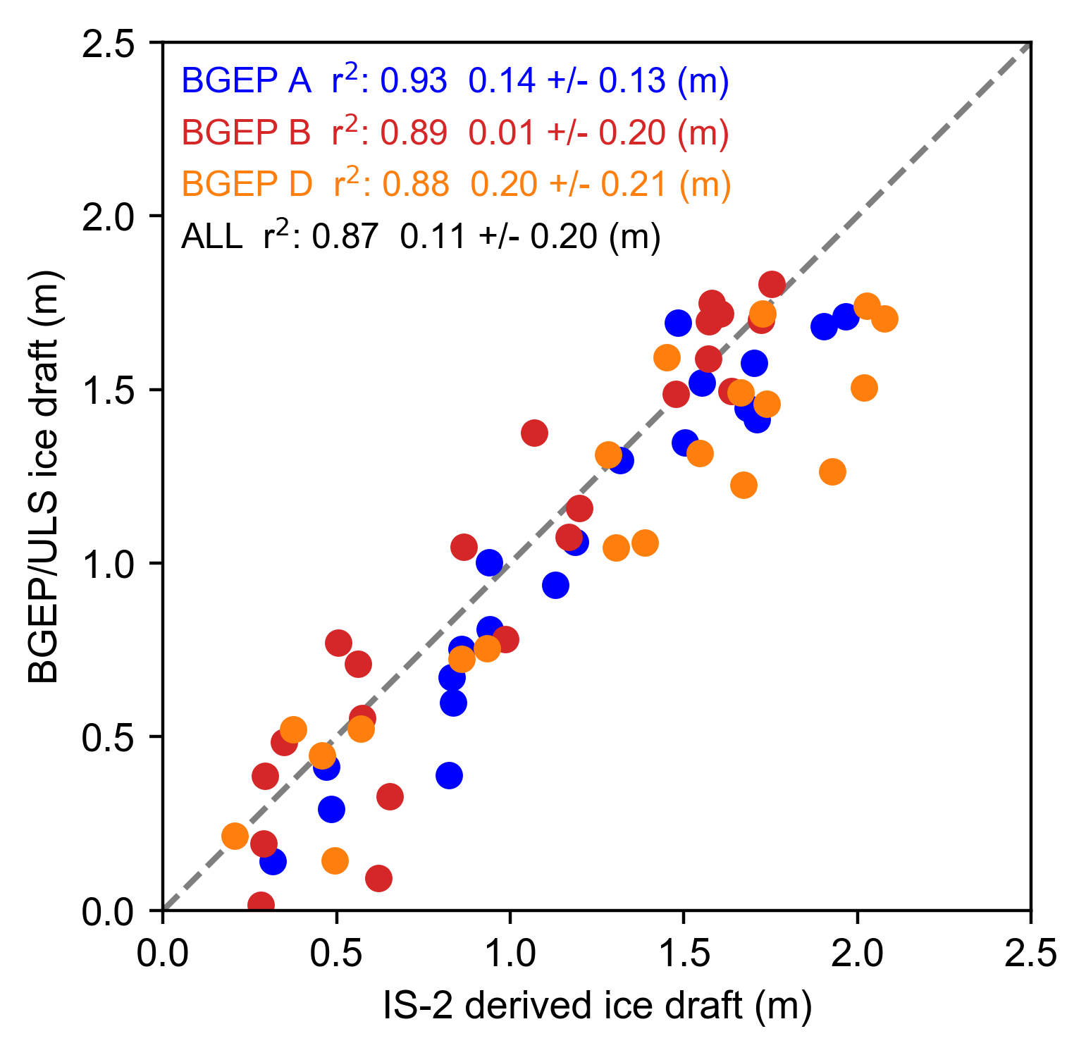
# Validation plot

plt.rc('font',**{'family':'sans-serif','sans-serif':['Arial']})
fig=plt.figure(figsize=(4, 4))
plt.scatter(monthly_IS2_at_ULS_a, uls_mean_monthly_draft_a_IS2_period, color='b')
plt.scatter(monthly_IS2_at_ULS_b, uls_mean_monthly_draft_b_IS2_period, color='tab:red')
plt.scatter(monthly_IS2_at_ULS_d, uls_mean_monthly_draft_d_IS2_period, color='tab:orange')
#plt.scatter(IS2_ULS_all, ULS_MONTHLY_IS2_all, color='k')

plt.annotate(r"BGEP A  r$^2$: "+r_str_a+"  "+mb_str_a+" +/- "+sd_str_a+" (m)", color='b', xy=(0.02, 0.98),xycoords='axes fraction', horizontalalignment='left', verticalalignment='top', fontsize=9)
plt.annotate(r"BGEP B  r$^2$: "+r_str_b+"  "+mb_str_b+" +/- "+sd_str_b+" (m)", color='tab:red', xy=(0.02, 0.92),xycoords='axes fraction', horizontalalignment='left', verticalalignment='top', fontsize=9)
plt.annotate(r"BGEP D  r$^2$: "+r_str_d+"  "+mb_str_d+" +/- "+sd_str_d+" (m)", color='tab:orange', xy=(0.02, 0.86),xycoords='axes fraction', horizontalalignment='left', verticalalignment='top', fontsize=9)
plt.annotate(r"ALL  r$^2$: "+r_str_all+"  "+mb_str_all+" +/- "+sd_str_all+" (m)", color='k', xy=(0.02, 0.80),xycoords='axes fraction', horizontalalignment='left', verticalalignment='top', fontsize=9)
        
plt.ylabel('BGEP/ULS ice draft (m)')
plt.xlabel('IS-2 derived ice draft (m)')
plt.xlim([0, 2.5])
plt.ylim([0, 2.5])
ax=plt.gca()
lims = [
    np.min([ax.get_xlim(), ax.get_ylim()]),  # min of both axes
    np.max([ax.get_xlim(), ax.get_ylim()]),  # max of both axes
]

# now plot both limits against each other
ax.plot(lims, lims, 'k--', alpha=0.5, zorder=0)
ax.set_aspect('equal')
ax.set_xlim(lims)
ax.set_ylim(lims)
plt.savefig('./figs/BGEP_scatter_res'+str(comp_res)+int_str+'_nn.pdf', dpi=200)
plt.show()

../_images/39391ec09a05d1aa9047407260fbd7a04715490d3c4a93245e304b0dad221f90.png

As a futher check, take a look at some maps to assess IS-2 coverage comapred to ULS locations, especially in the early season#

uls_x_a, uls_y_a = mapProj(-150., 75.)
uls_x_b, uls_y_b = mapProj(-150., 78.4)
uls_x_d, uls_y_d = mapProj(-140., 74.)

date = "Sep 2019"
var = "ice_thickness"+int_str
data_one_month = book_ds[var].sel(time=date)
p = data_one_month.plot(x="longitude", y="latitude", # horizontal coordinates 
                        vmin=0, vmax=4, # min and max on the colorbar 
                        subplot_kws={'projection':ccrs.NorthPolarStereo(central_longitude=-45)}, # Set the projection 
                        transform=ccrs.PlateCarree())

plt.plot(uls_x_a, uls_y_a, '.', color='b', transform=ccrs.NorthPolarStereo(central_longitude=-45))
plt.plot(uls_x_b, uls_y_b, '.', color='m', transform=ccrs.NorthPolarStereo(central_longitude=-45))
plt.plot(uls_x_d, uls_y_d, '.', color='k', transform=ccrs.NorthPolarStereo(central_longitude=-45))

plt.text(uls_x_a, uls_y_a, 'A', color='b', transform=ccrs.NorthPolarStereo(central_longitude=-45))
plt.text(uls_x_b, uls_y_b, 'B', color='m', transform=ccrs.NorthPolarStereo(central_longitude=-45))
plt.text(uls_x_d, uls_y_d, 'D', color='k', transform=ccrs.NorthPolarStereo(central_longitude=-45))


p.axes.coastlines() # Add coastlines 
plt.show()

../_images/ba932893f4564142b191c95f43cfa15676204f966d2e9aa6e2d4e3890eb1fe3a.png

Comparisons with BGEP ULS sea ice draft estimates

Contents

Comparisons with BGEP ULS sea ice draft estimates#

Import notebook dependencies#

As a futher check, take a look at some maps to assess IS-2 coverage comapred to ULS locations, especially in the early season#