Winter Arctic sea ice state variability#
Summary: In this notebook, we highlight key additional sea ice variables: snow depth, ice type, snow density, and sea ice drift. We’ll use cartopy and xarray to generate maps and lineplots of the data to demonstrate methods for visualizing the data statically, as opposed to the interactive plotting functions highlighted in the seperate interactive notebooks (which can be slow to render and push the GitHub file size limits!).
Please take a look at the ‘Data variables’ tab in the book_ds cell below to explore the potential variables for analysis in this notebook.
The dataset also includes a few interpolated/smoothed variables (freeboard_int, snow_depth_int, ice_thickness_int) that can be used instead of the raw monthly means to increase coverage in some regions. See the interp_demo notebook for more information on how they are derived.
The analysis presented here was peer-reviewed in this paper in The Cryosphere.
Version history: Version 1 (01/01/2022)
Import notebook dependencies#
# For working with gridded climate data
import xarray as xr
# Helper function for reading the data from the bucket
from utils.read_data_utils import read_book_data
from utils.plotting_utils import static_winter_comparison_lineplot, staticArcticMaps, staticArcticMaps_overlayDrifts, interactiveArcticMaps, compute_gridcell_winter_means # Plotting utils
import numpy as np
# Plotting dependencies
#%config InlineBackend.figure_format = 'retina'
import matplotlib as mpl
# Sets figure size in the notebook
mpl.rcParams['figure.dpi'] = 150

# Remove warnings to improve display
import warnings
warnings.filterwarnings('ignore')
# Set some plotting parameters
mpl.rcParams.update({
    "text.usetex": False,  # Use LaTeX for rendering
    "font.family": "sans-serif",
    'mathtext.fontset': 'stixsans',
    "lines.linewidth": 1.,
    "font.size": 8,
    #"lines.alpha": 0.8,
    "axes.labelsize": 8,
    "xtick.labelsize": 8,
    "ytick.labelsize": 8,
    "legend.fontsize": 8
})
mpl.rcParams['font.sans-serif'] = ['Arial']
mpl.rcParams['figure.dpi'] = 300
Read in the aggregated monthly gridded winter Arctic sea ice data#
book_ds = read_book_data() # Read/download the data
book_ds
<xarray.Dataset> Size: 345MB
Dimensions:               (time: 30, y: 448, x: 304)
Coordinates:
  * time                  (time) datetime64[ns] 240B 2018-11-01 ... 2021-04-01
    longitude             (y, x) float32 545kB ...
    latitude              (y, x) float32 545kB ...
    xgrid                 (y, x) float32 545kB ...
    ygrid                 (y, x) float32 545kB ...
Dimensions without coordinates: y, x
Data variables: (12/20)
    projection            (time) float64 240B ...
    ice_thickness         (time, y, x) float32 16MB ...
    ice_thickness_unc     (time, y, x) float32 16MB ...
    num_segments          (time, y, x) float32 16MB ...
    mean_day_of_month     (time, y, x) float32 16MB ...
    snow_depth            (time, y, x) float32 16MB ...
    ...                    ...
    region_mask           (time, y, x) float32 16MB ...
    piomas_ice_thickness  (time, y, x) float32 16MB ...
    t2m                   (time, y, x) float32 16MB ...
    msdwlwrf              (time, y, x) float32 16MB ...
    x_vel                 (time, y, x) float64 33MB ...
    y_vel                 (time, y, x) float64 33MB ...
Attributes:
    contact:      Alek Petty (alek.a.petty@nasa.gov)
    description:  Gridded Oct 2019 Arctic sea ice thickness and ancillary dat...
    reference:    Data doi: 10.5067/CV6JEXEE31HF. Original methodology descri...
history: Created 21/01/22Static winter mean maps#
Compute and map (static) gridcell winter means for given variables
years = [2018,2019,2020] # Years over which to perform analysis

print(compute_gridcell_winter_means.__doc__) # Print docstring
print(staticArcticMaps.__doc__) # Print docstring
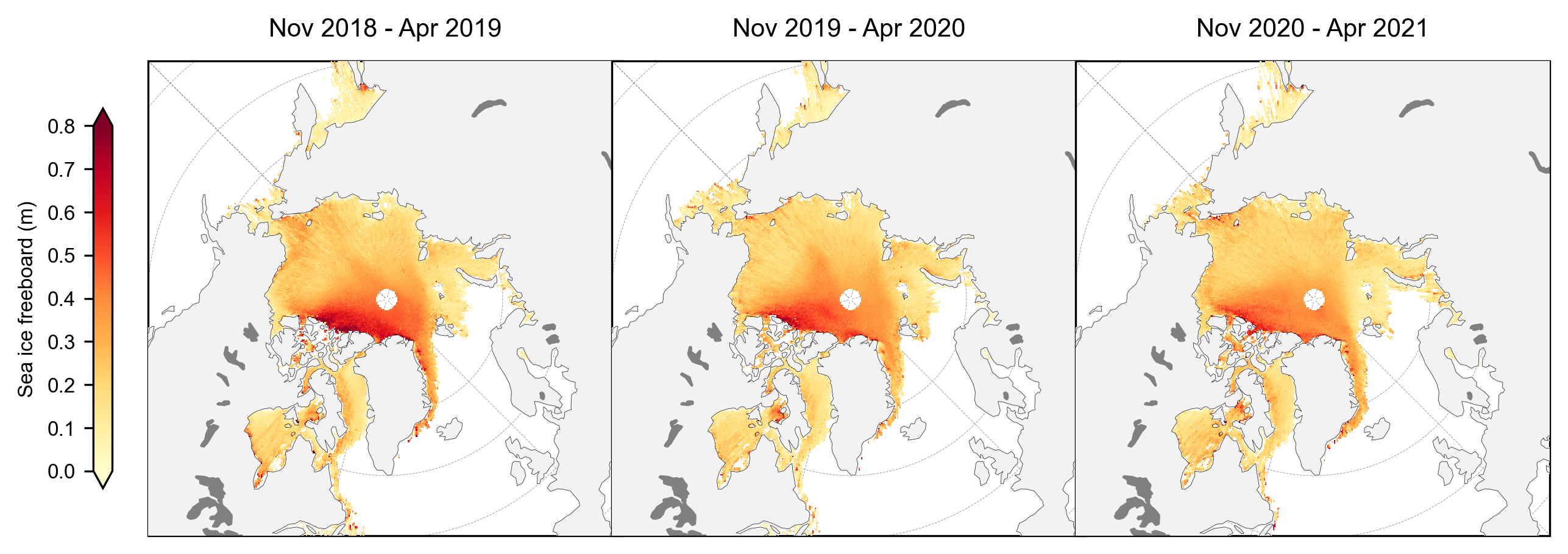
freeboard_winter_means = compute_gridcell_winter_means(book_ds.freeboard, years=years)
staticArcticMaps(freeboard_winter_means, dates=freeboard_winter_means.time.values, set_cbarlabel = "Sea ice freeboard (m)", cmap="YlOrRd", vmin=0, vmax=0.8, out_str='freeboard_winter')
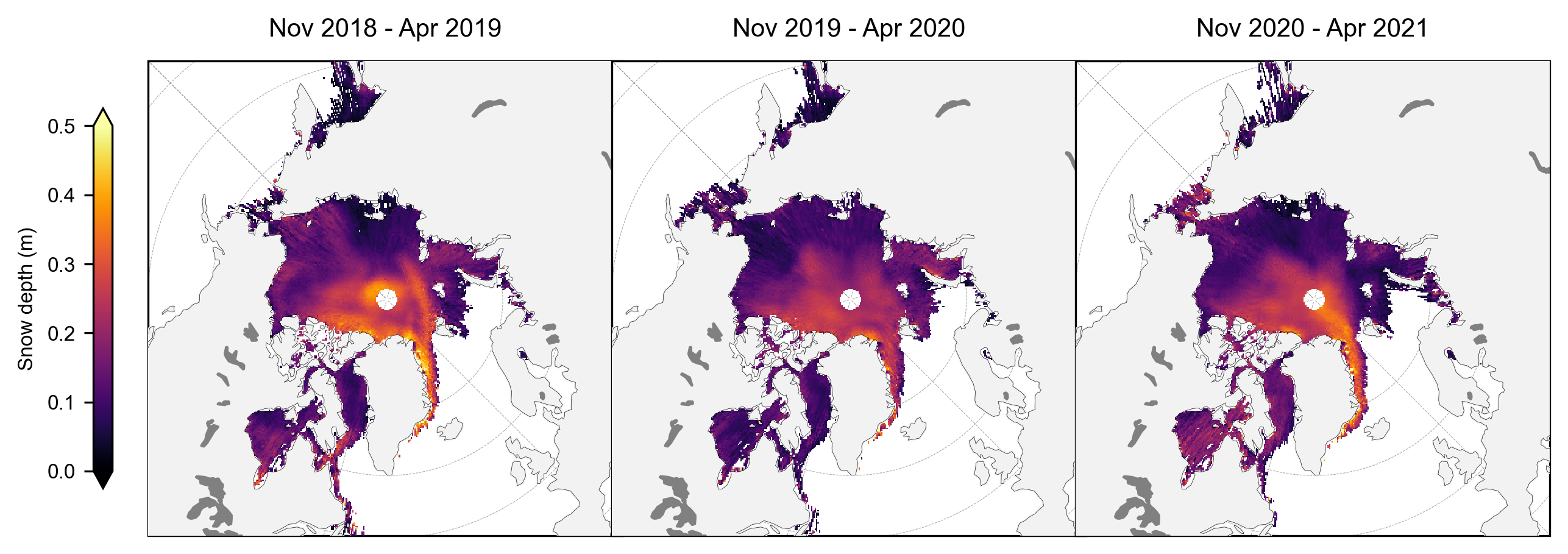
snow_depth_winter_means = compute_gridcell_winter_means(book_ds.snow_depth, years=years)
staticArcticMaps(snow_depth_winter_means, dates=snow_depth_winter_means.time.values, set_cbarlabel = "Snow depth (m)", cmap="inferno", vmin=0, vmax=0.5, out_str='snowdepth_winter')
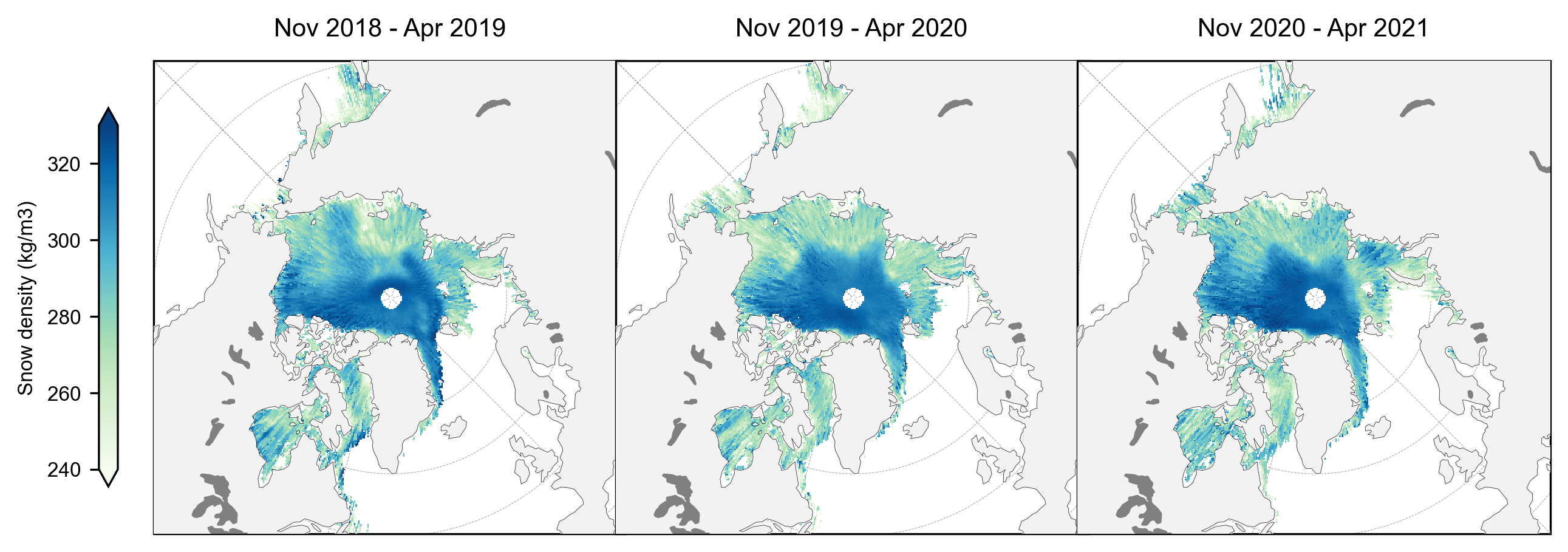
snow_density_winter_means = compute_gridcell_winter_means(book_ds.snow_density, years=years)
staticArcticMaps(snow_density_winter_means, dates=snow_depth_winter_means.time.values, set_cbarlabel = "Snow density (kg/m3)", cmap="GnBu", vmin=240, vmax=330, out_str='snowdensity_winter')
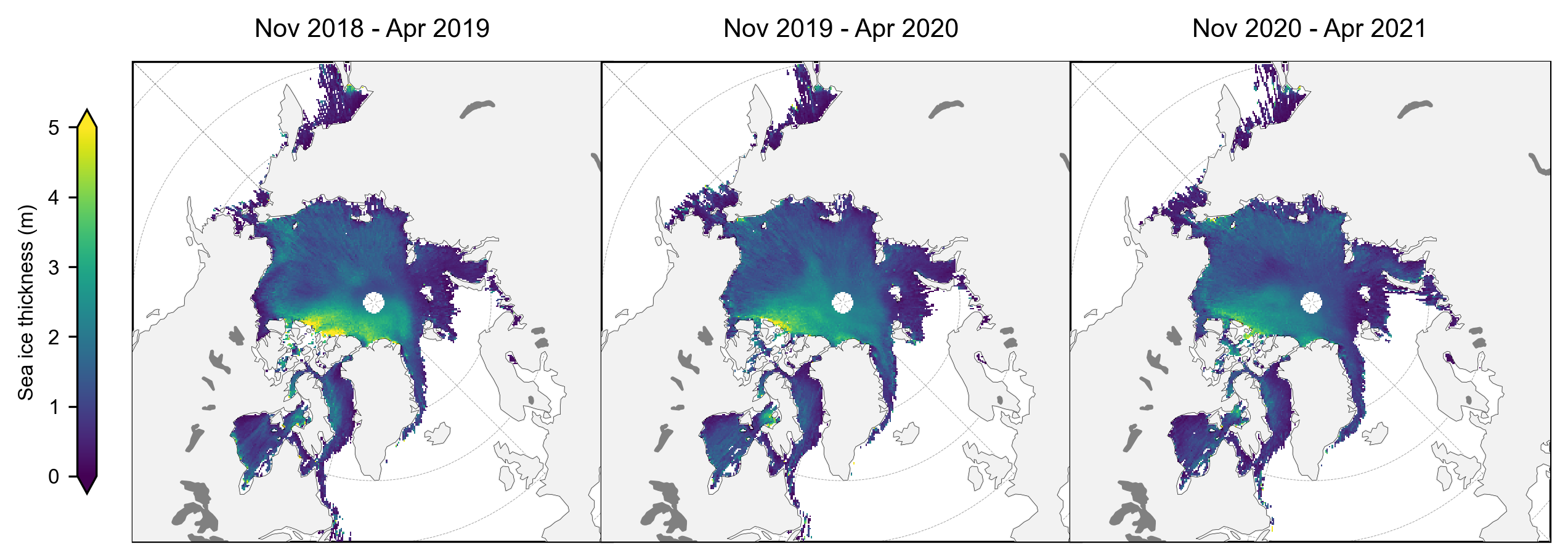
thickness_winter_means = compute_gridcell_winter_means(book_ds.ice_thickness, years=years)
staticArcticMaps(thickness_winter_means, dates=thickness_winter_means.time.values, title="", set_cbarlabel = "Sea ice thickness (m)", cmap="viridis", vmin=0, vmax=5, out_str='thickness_winter')
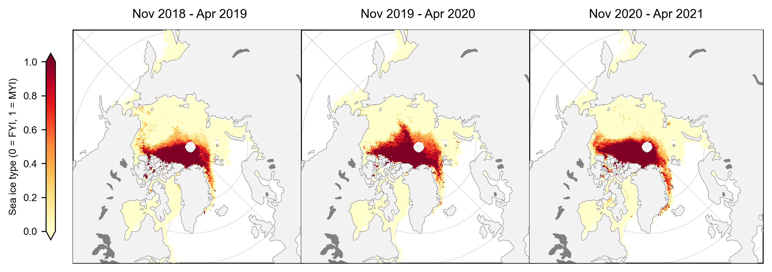
ice_type_winter_means = compute_gridcell_winter_means(book_ds.ice_type, years=years)
staticArcticMaps(ice_type_winter_means, dates=ice_type_winter_means.time.values, set_cbarlabel = "Sea ice type (0 = FYI, 1 = MYI)", cmap="YlOrRd", vmin=0, vmax=1, out_str='icetype_winter')
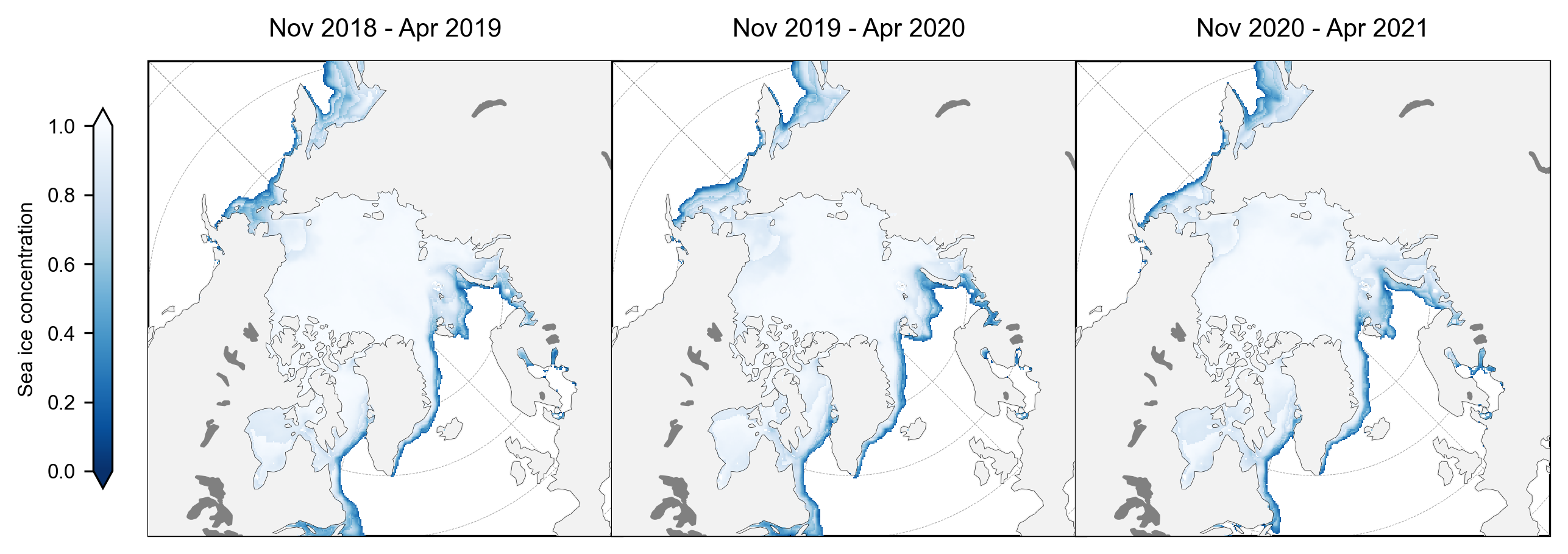
ice_conc_winter_means = compute_gridcell_winter_means(book_ds.sea_ice_conc, years=years)
staticArcticMaps(ice_conc_winter_means, dates=ice_conc_winter_means.time.values, set_cbarlabel = "Sea ice concentration", cmap="Blues_r", vmin=0, vmax=1, out_str='iceconc_winter')
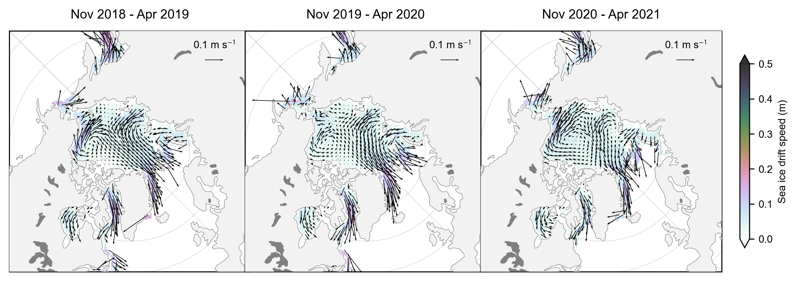
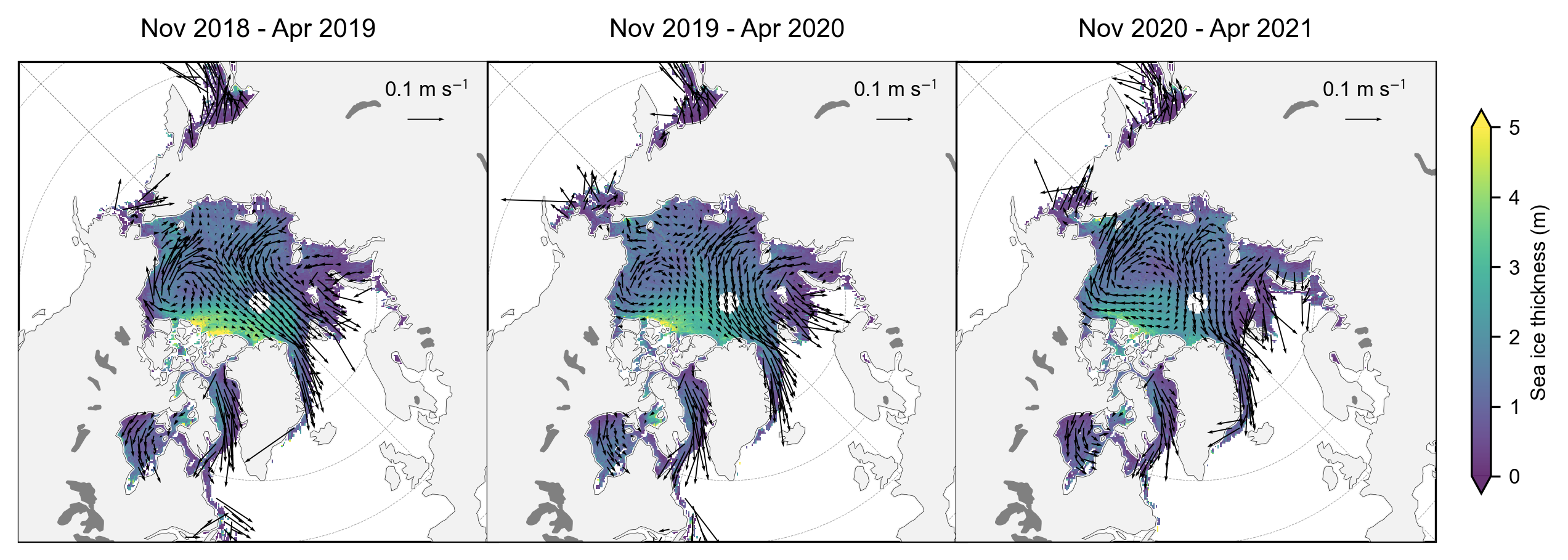
Overlay sea ice drift vectors#
We can use a modified version of the plotting function used above to overlay sea ice drift vectors on any variable of interest. Below, we’ll generate the plot presented in Petty et al. (2022) that shows mean sea ice thickness and mean sea ice drift for the three winters.
print(staticArcticMaps_overlayDrifts.__doc__)
# Compute winter means

drifts_xvel_winter_means = compute_gridcell_winter_means(book_ds.x_vel, years=years)
drifts_yvel_winter_means = compute_gridcell_winter_means(book_ds.y_vel, years=years)
drifts_mag_winter_means = compute_gridcell_winter_means(np.sqrt(book_ds.x_vel**2+book_ds.y_vel**2).rename('mag'), years=years)

# Generate plot
staticArcticMaps_overlayDrifts(da=drifts_mag_winter_means,
                                           dates=drifts_mag_winter_means.time.values,
                                           drifts_x=drifts_xvel_winter_means,
                                           drifts_y=drifts_yvel_winter_means,
                                           set_cbarlabel="Sea ice drift speed (m)", cmap="cubehelix_r",
                                           vmin=0, vmax=0.5, alpha=0.8, res = 6,
                                           out_str='driftmag_drifts_overlayed')
# Compute winter means
thickness_winter_means = compute_gridcell_winter_means(book_ds.ice_thickness, years=years)
drifts_xvel_winter_means = compute_gridcell_winter_means(book_ds.x_vel, years=years)
drifts_yvel_winter_means = compute_gridcell_winter_means(book_ds.y_vel, years=years)

# Generate plot
pl_drifts = staticArcticMaps_overlayDrifts(da=thickness_winter_means,
                                           dates=thickness_winter_means.time.values,
                                           drifts_x=drifts_xvel_winter_means,
                                           drifts_y=drifts_yvel_winter_means,
                                           set_cbarlabel="Sea ice thickness (m)", cmap="viridis",
                                           vmin=0, vmax=5, alpha=0.8,
                                           out_str='thickness_drifts_overlayed')
display(pl_drifts)
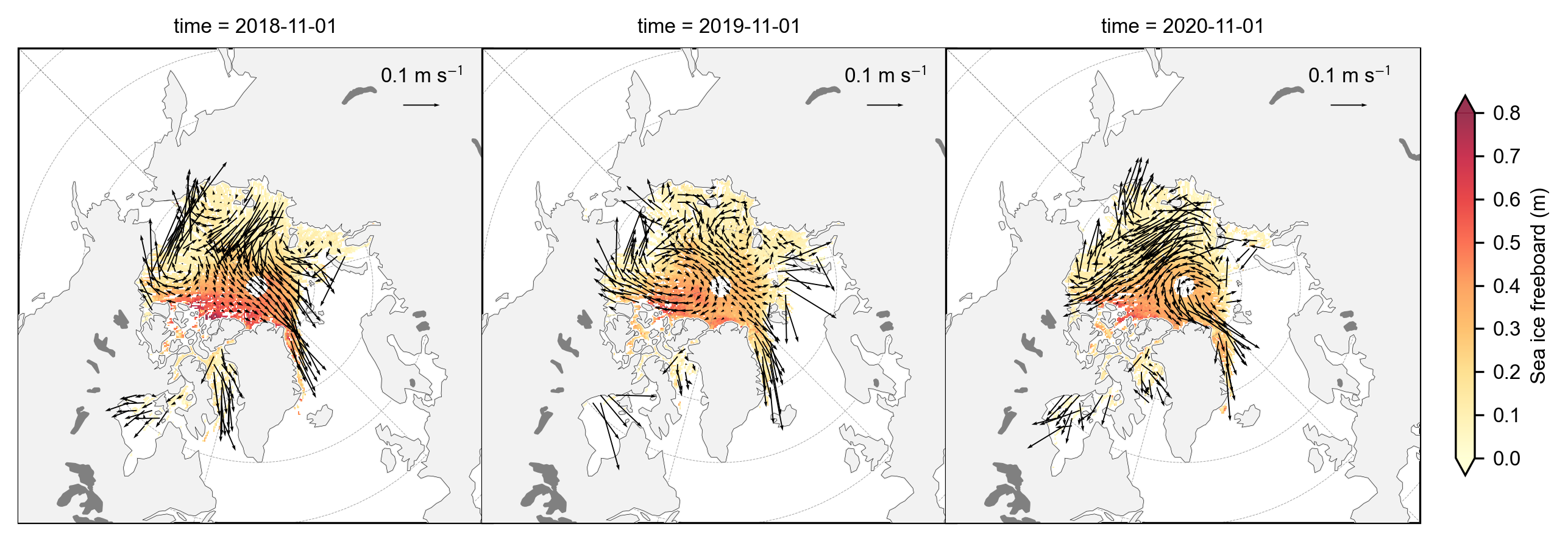
You can also plot the sea ice drifts for just a single month. Below, we’ll show November sea ice drift overlayed on November sea ice freeboard for three winter seasons.
# Generate plot
pl_drifts = staticArcticMaps_overlayDrifts(da=book_ds.freeboard.sel(time=["Nov 2018","Nov 2019","Nov 2020"]),
                                           drifts_x=book_ds.x_vel.sel(time=["Nov 2018","Nov 2019","Nov 2020"]),
                                           drifts_y=book_ds.y_vel.sel(time=["Nov 2018","Nov 2019","Nov 2020"]),
                                           set_cbarlabel="Sea ice freeboard (m)", cmap="YlOrRd",
                                           vmin=0, vmax=0.8, alpha=0.8,
                                           out_str='nov_freeboard_drifts_overlayed')
display(pl_drifts)
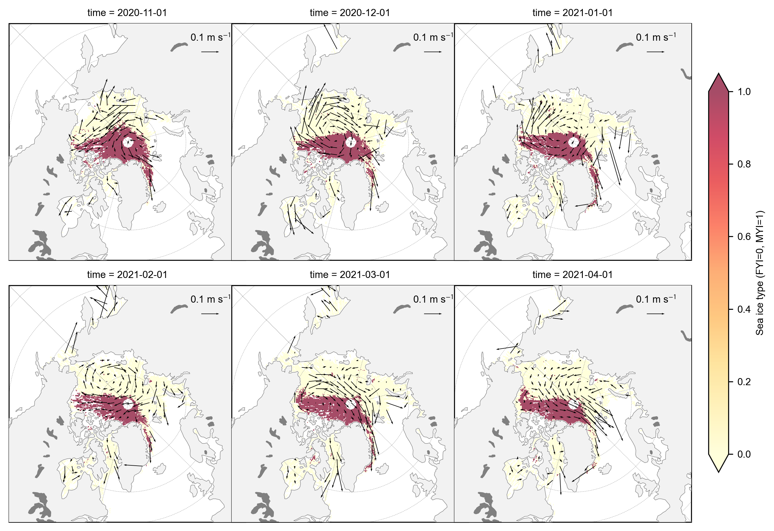
We can also change the resolution of the drifts to see more or less detail in the overlaid vectors. You can do this by changing the res argument, set to a default of 6. You also might want to change the opacity of the data to improve the visualization, which can be altered with the alpha argument. Setting alpha=1 indicates you want full opacity, and less than 1 indicates for some degree of transparency.
Below, we’ll plot sea ice type with an alpha of 0.7 and a drift vector resoltion of 11 (display 1 out of every 11 vectors).
# Generate plot
pl_drifts = staticArcticMaps_overlayDrifts(da=book_ds.ice_type.sel(time=slice("Nov 2020", "April 2021")),
                                           drifts_x=book_ds.x_vel.sel(time=slice("Nov 2020", "April 2021")),
                                           drifts_y=book_ds.y_vel.sel(time=slice("Nov 2020", "April 2021")),
                                           set_cbarlabel="Sea ice type (FYI=0, MYI=1)", cmap="YlOrRd",
                                           vmin=0, vmax=1, alpha=0.7, res = 11,
                                           out_str='ice_type_drifts_overlayed')
display(pl_drifts)
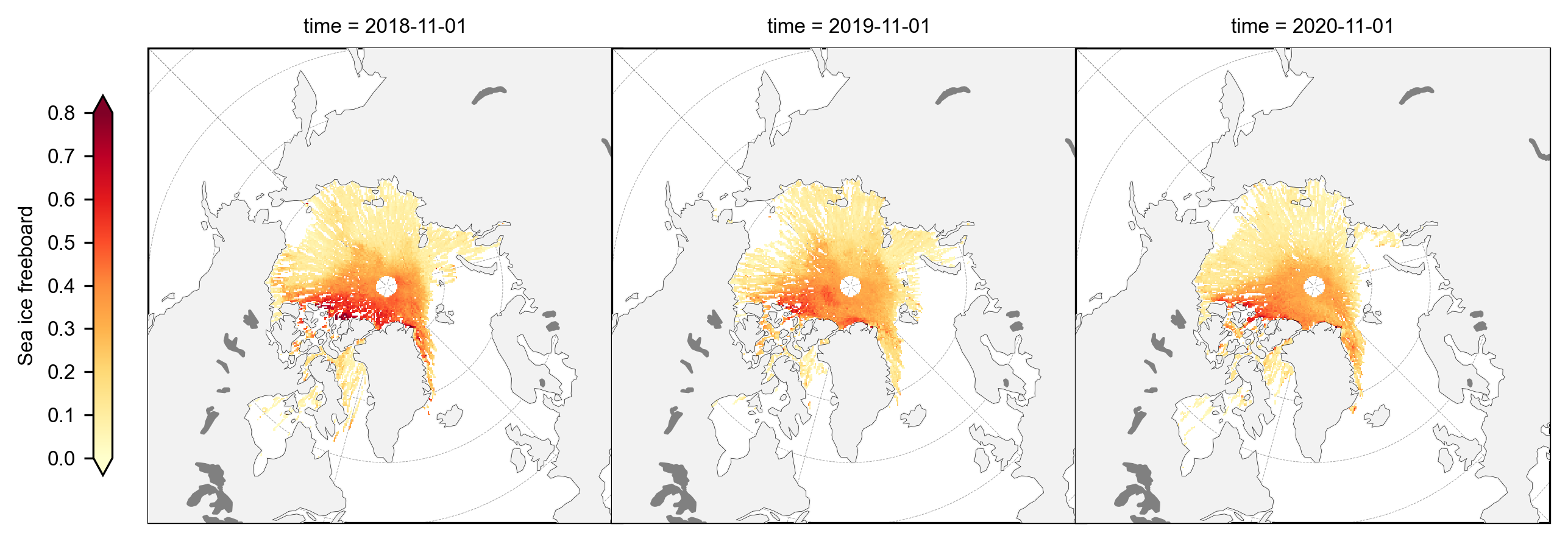
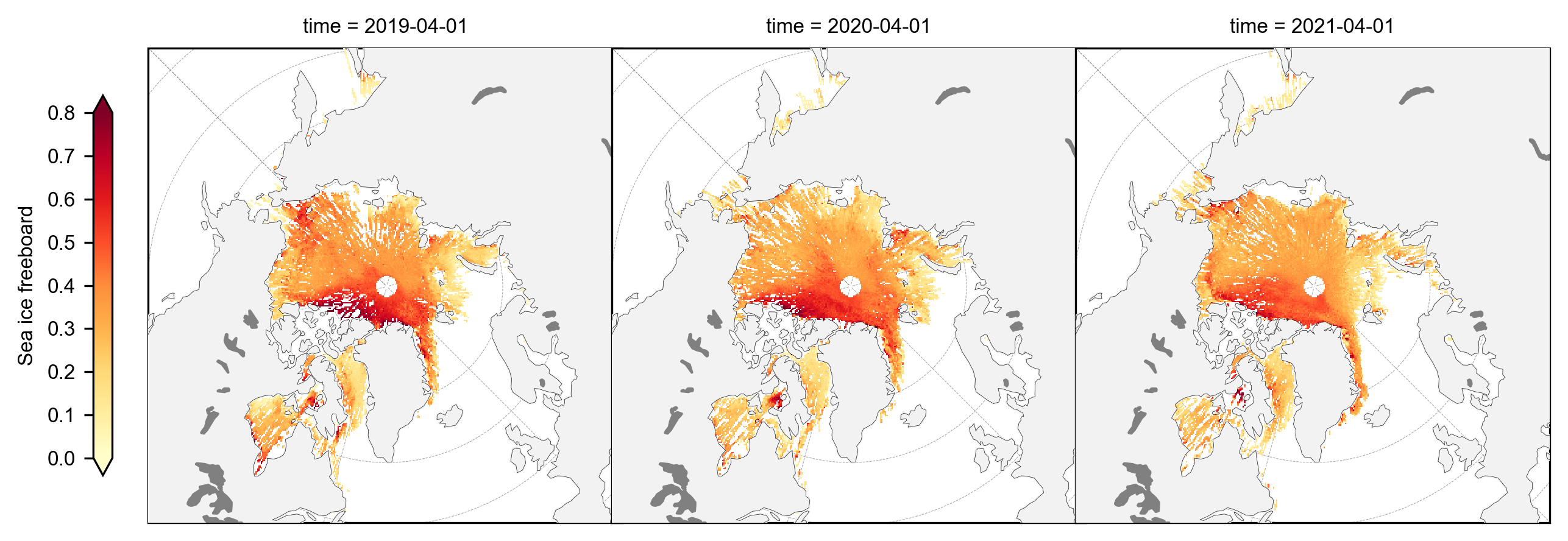
Static monthly maps#
Compute and map (static) data given variables across the three winters for individual months
pl = staticArcticMaps(book_ds.freeboard.sel(time=["Nov 2018","Nov 2019","Nov 2020"]), set_cbarlabel = "Sea ice freeboard", cmap="YlOrRd", vmin=0, vmax=0.8, out_str='freeboard_november')
display(pl)
pl = staticArcticMaps(book_ds.freeboard.sel(time=["Apr 2019","Apr 2020","Apr 2021"]), set_cbarlabel = "Sea ice freeboard", cmap="YlOrRd", vmin=0, vmax=0.8, out_str='freeboard_april')
display(pl)
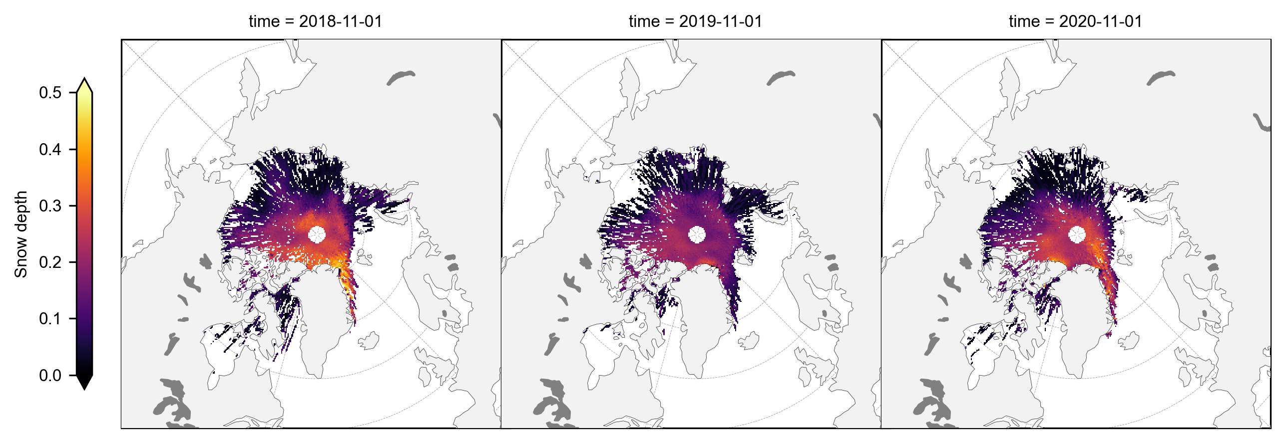
pl = staticArcticMaps(book_ds.snow_depth.sel(time=["Nov 2018","Nov 2019","Nov 2020"]), set_cbarlabel = "Snow depth", cmap="inferno", vmin=0, vmax=0.5, out_str='snowdepth_november')
display(pl)
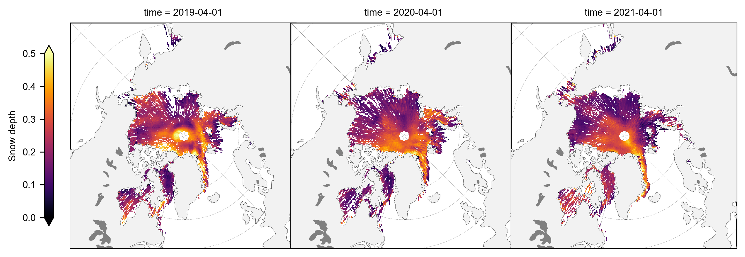
pl = staticArcticMaps(book_ds.snow_depth.sel(time=["Apr 2019","Apr 2020","Apr 2021"]), set_cbarlabel = "Snow depth", cmap="inferno", vmin=0, vmax=0.5, out_str='snowdepth_april')
display(pl)
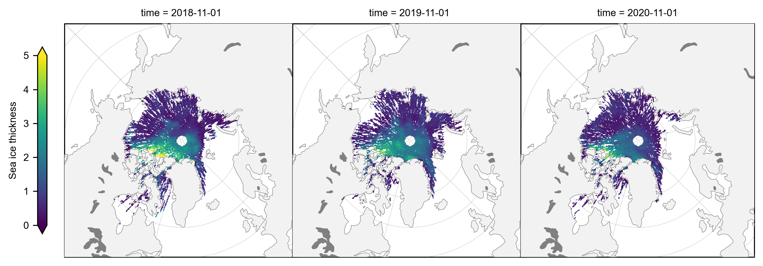
pl = staticArcticMaps(book_ds.ice_thickness.sel(time=["Nov 2018","Nov 2019","Nov 2020"]), set_cbarlabel = "Sea ice thickness", cmap="viridis", vmin=0, vmax=5, out_str='thickness_november')
display(pl)
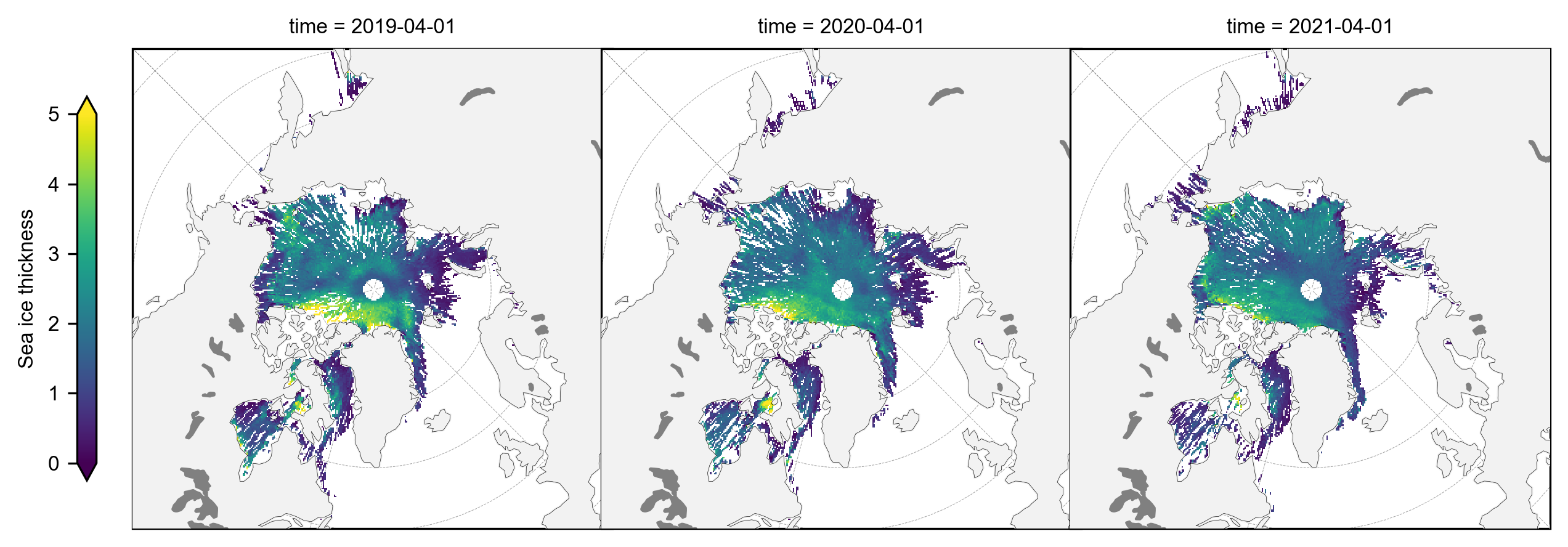
pl = staticArcticMaps(book_ds.ice_thickness.sel(time=["Apr 2019","Apr 2020","Apr 2021"]), set_cbarlabel = "Sea ice thickness", cmap="viridis", vmin=0, vmax=5, out_str='thickness_april')
display(pl)
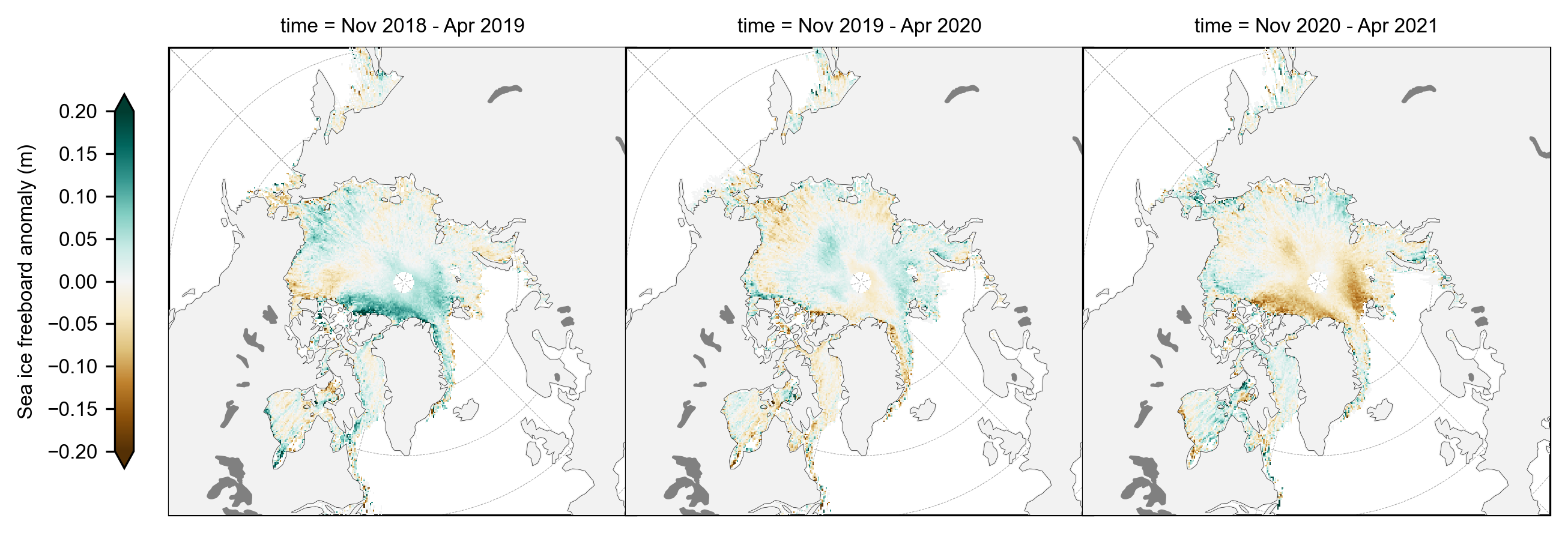
Thickness anomaly plots#
Compute and map (static) monthly anomaly maps (relative to the mean across the three winters by default) for given variables across the three winters
freeboard_winter_means = compute_gridcell_winter_means(book_ds.freeboard, years=years)
pl = staticArcticMaps(freeboard_winter_means-freeboard_winter_means.mean(axis=0), title="", set_cbarlabel = "Sea ice freeboard anomaly (m)", cmap="BrBG", vmin=-0.2, vmax=0.2, out_str='freeboard_winter_anomaly')
display(pl)
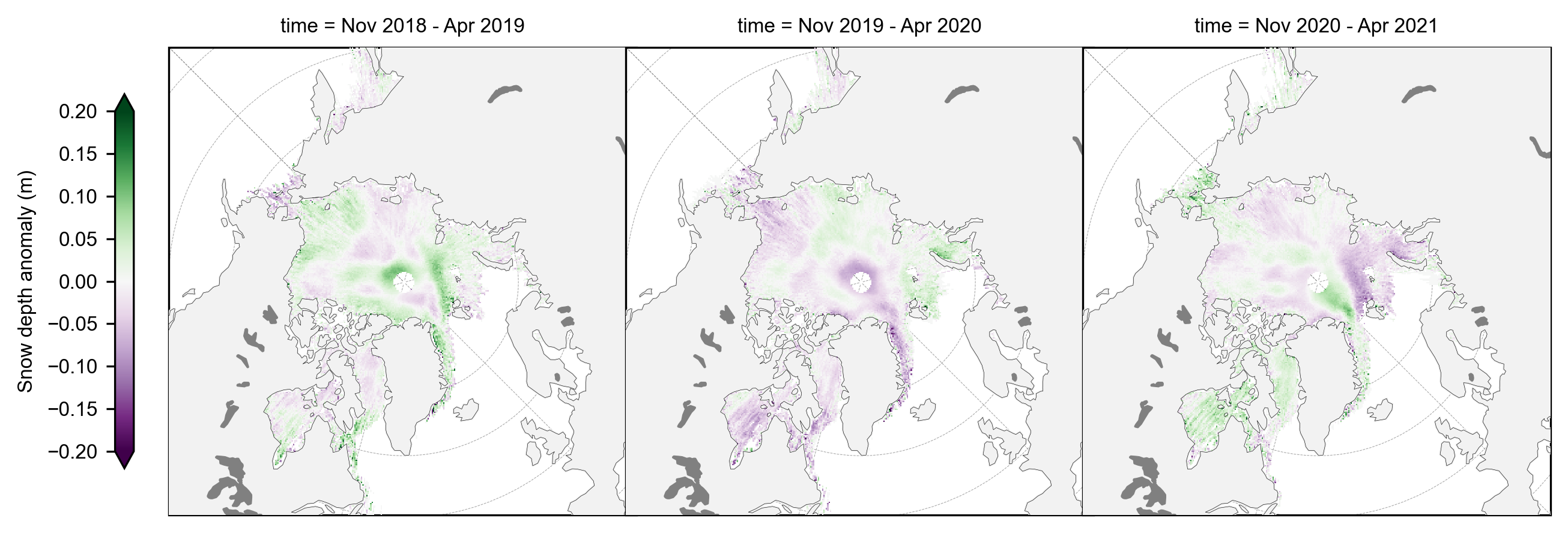
snow_depth_winter_means = compute_gridcell_winter_means(book_ds.snow_depth, years=years)
pl = staticArcticMaps(snow_depth_winter_means-snow_depth_winter_means.mean(axis=0), set_cbarlabel = "Snow depth anomaly (m)", cmap="PRGn", vmin=-0.2, vmax=0.2, out_str='snowdepth_winter_anomaly')
display(pl)
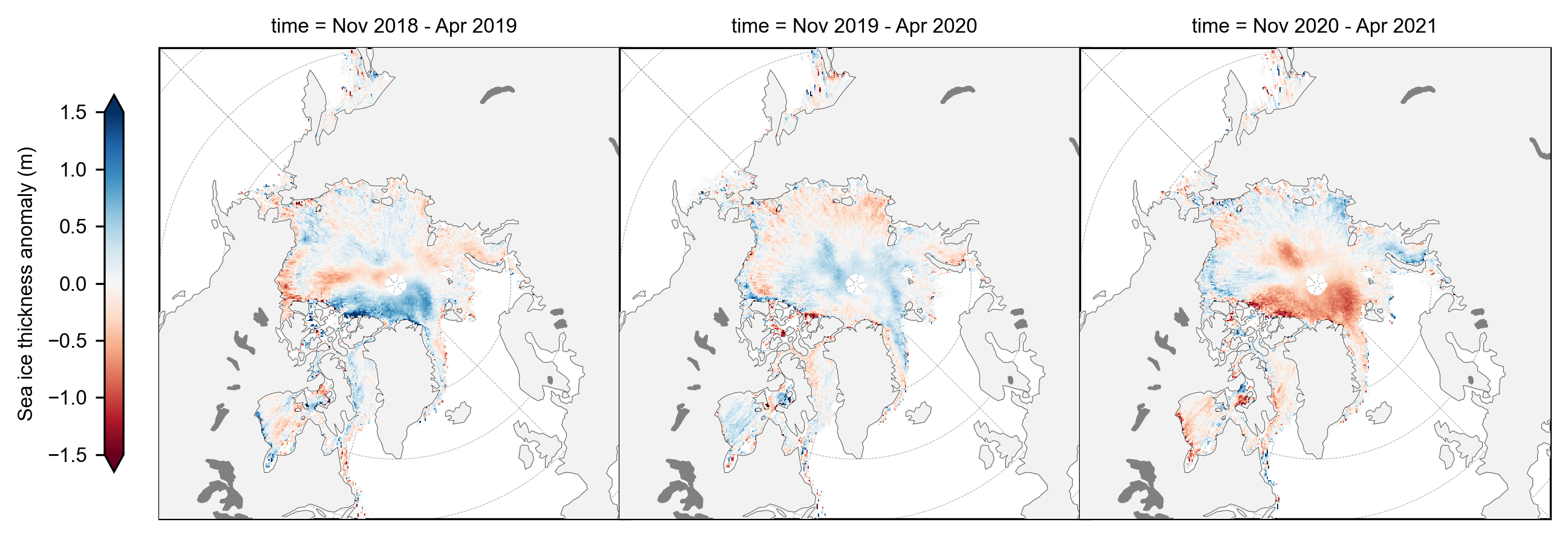
thickness_winter_means = compute_gridcell_winter_means(book_ds.ice_thickness, years=years)
pl = staticArcticMaps(thickness_winter_means-thickness_winter_means.mean(axis=0), set_cbarlabel = "Sea ice thickness anomaly (m)", cmap="RdBu", vmin=-1.5, vmax=1.5, out_str='thickness_winter_anomaly')
display(pl)
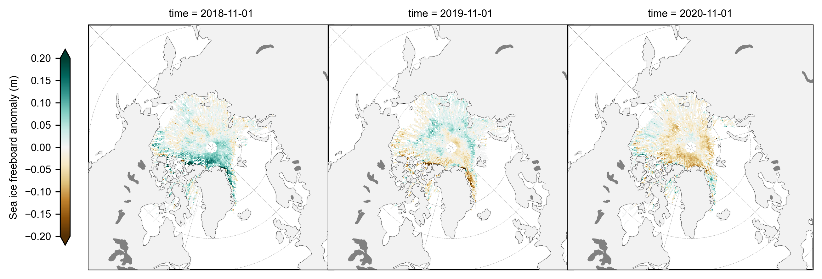
Do the same for the monthly anomalies (November then April)
pl = staticArcticMaps(book_ds.freeboard[0::12]-book_ds.freeboard[0::12].mean(axis=0), set_cbarlabel = "Sea ice freeboard anomaly (m)", cmap="BrBG", vmin=-0.2, vmax=0.2, out_str='freeboard_november_anomaly')
display(pl)
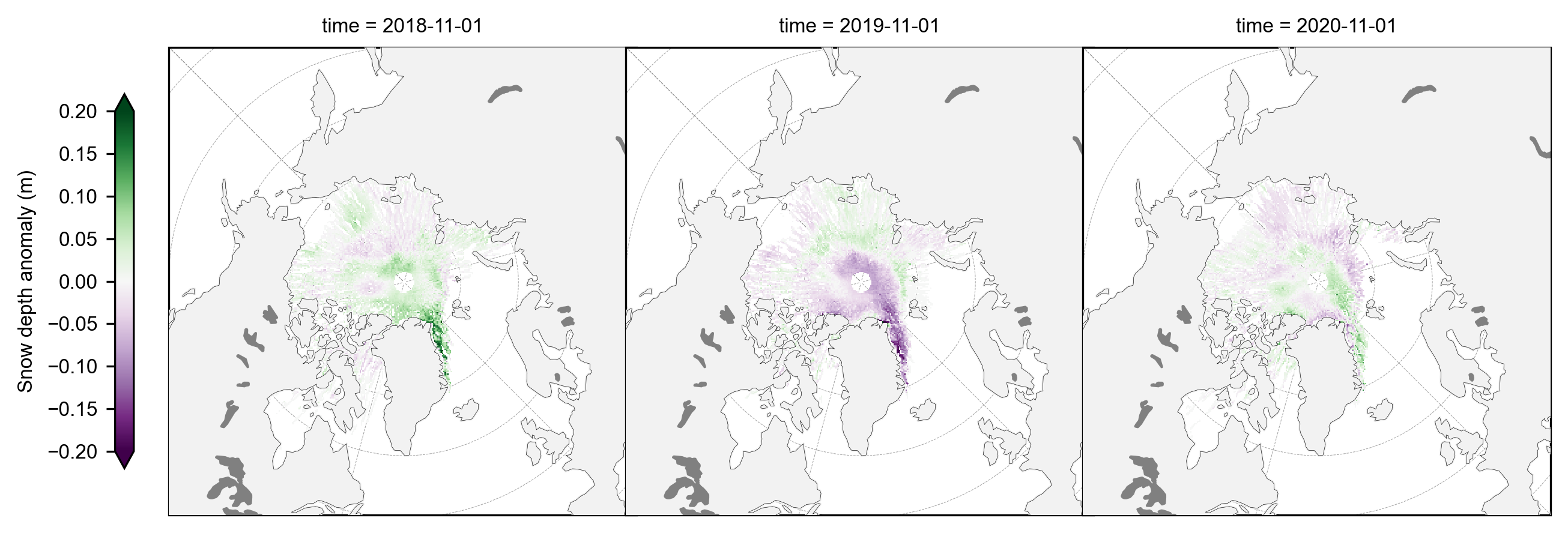
pl = staticArcticMaps(book_ds.snow_depth[0::12]-book_ds.snow_depth[0::12].mean(axis=0), set_cbarlabel = "Snow depth anomaly (m)", cmap="PRGn", vmin=-0.2, vmax=0.2, out_str='snow_depth_november_anomaly')
display(pl)
pl = staticArcticMaps(book_ds.ice_thickness[5::12]-book_ds.ice_thickness[5::12].mean(axis=0), set_cbarlabel = "Sea ice thickness anomaly (m)", cmap="RdBu", vmin=-1.5, vmax=1.5, out_str='thickness_november_anomaly')
display(pl)
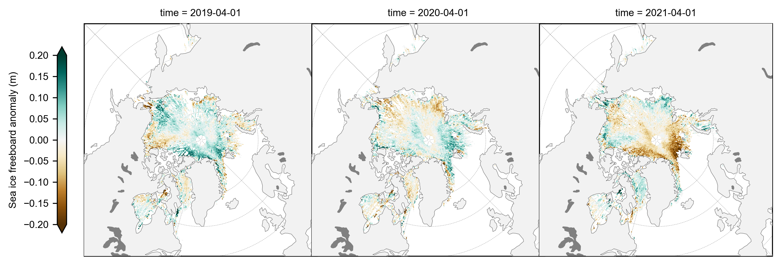
pl = staticArcticMaps(book_ds.freeboard[5::12]-book_ds.freeboard[5::12].mean(axis=0), set_cbarlabel = "Sea ice freeboard anomaly (m)", cmap="BrBG", vmin=-0.2, vmax=0.2, out_str='freeboard_april_anomaly')
display(pl)
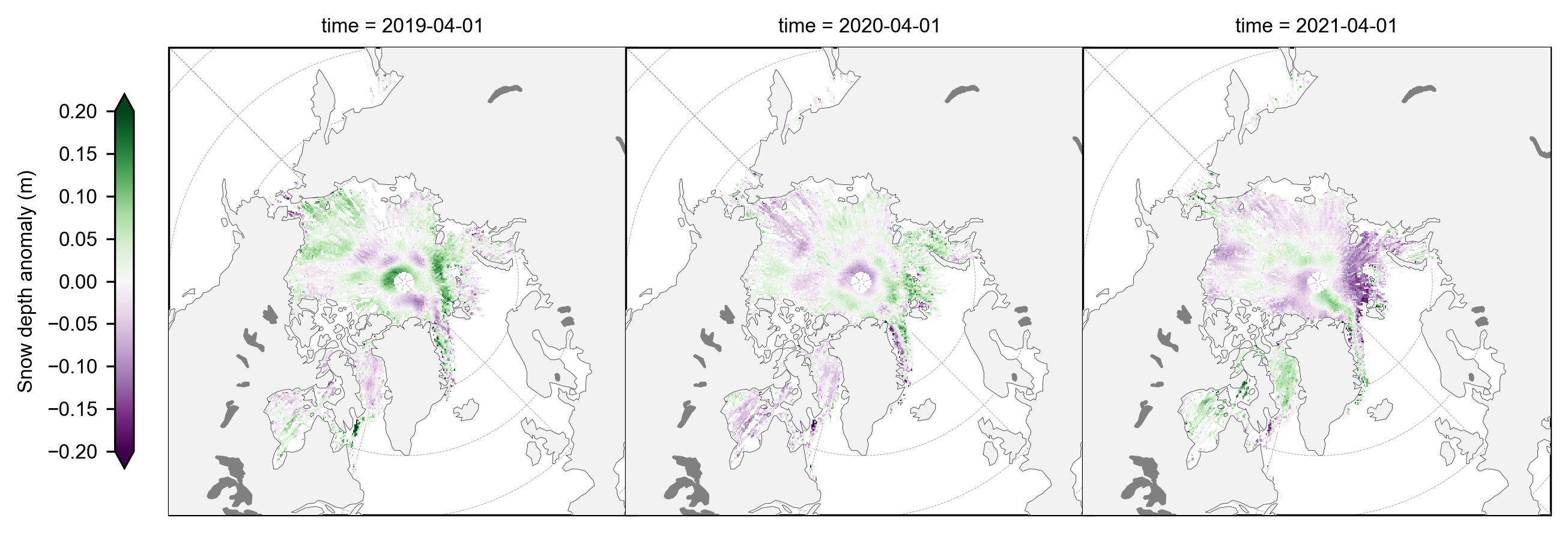
pl = staticArcticMaps(book_ds.snow_depth[5::12]-book_ds.snow_depth[5::12].mean(axis=0), set_cbarlabel = "Snow depth anomaly (m)", cmap="PRGn", vmin=-0.2, vmax=0.2, out_str='snow_depth_april_anomaly')
display(pl)
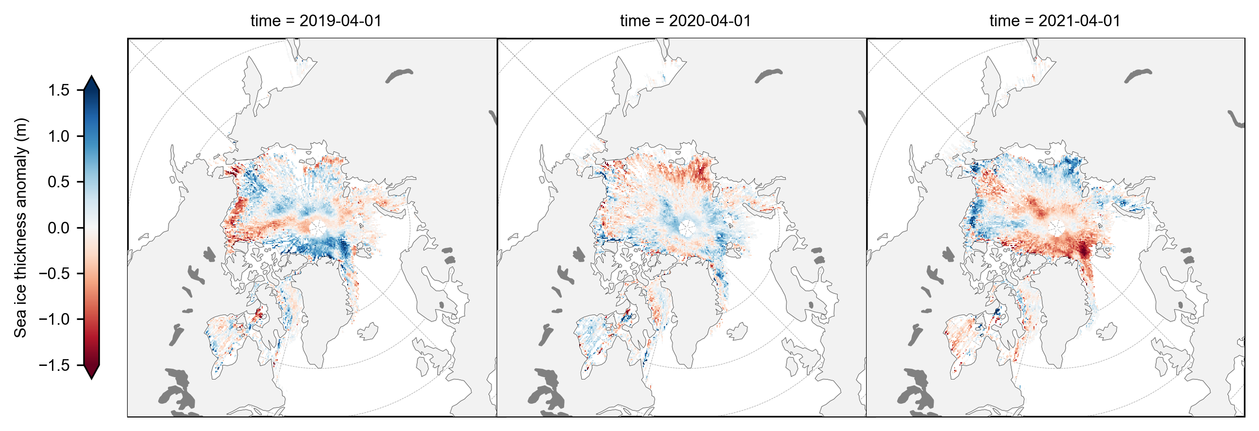
pl = staticArcticMaps(book_ds.ice_thickness[5::12]-book_ds.ice_thickness[5::12].mean(axis=0), set_cbarlabel = "Sea ice thickness anomaly (m)", cmap="RdBu", vmin=-1.5, vmax=1.5, out_str='thickness_april_anomaly')
display(pl)
Monthly mean timeseries#
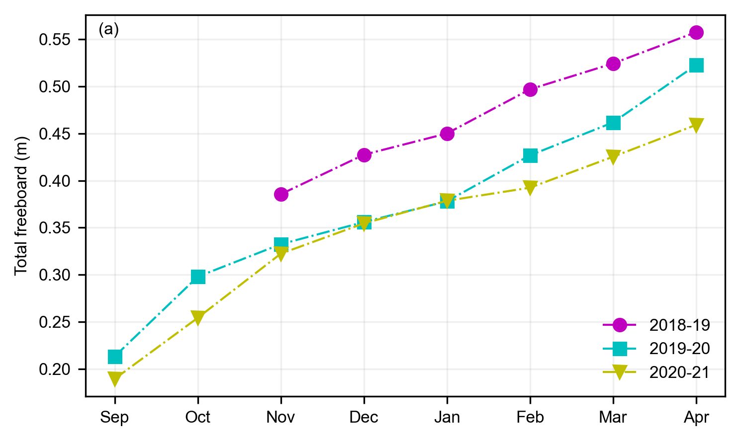
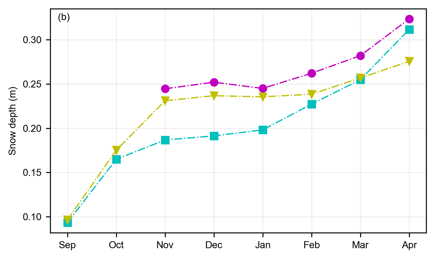
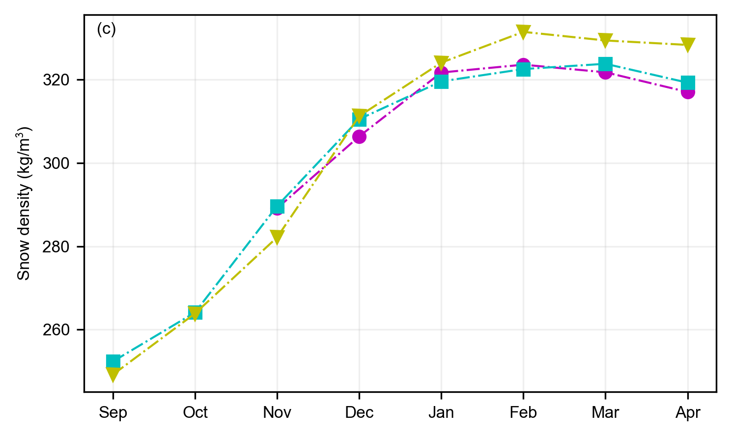
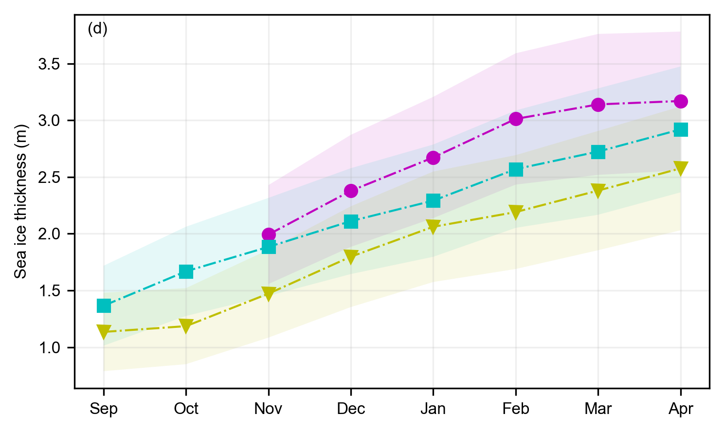
Next we’ll compute monthly means by averaging over all gridcells within a given region. We’ll use this to generate a lineplot to compare across the three winter seasons for each variable.
# Here is where we might also want to set a region mask, e.g. to avoid including some of the more uncertain data in the peripheral seas
innerArctic = [1,2,3,4,5,6]
book_ds_innerArctic = book_ds.where(book_ds.region_mask.isin(innerArctic))

# Uncomment out to set an additional ice type mask too and change the save_label accordingly (0 = FYI, 1 = MYI)
book_ds_innerArctic = book_ds_innerArctic.where(book_ds_innerArctic.ice_type==1)

save_label='Inner_Arctic_MYI'
print(static_winter_comparison_lineplot.__doc__) # Print docstring
static_winter_comparison_lineplot(book_ds_innerArctic.freeboard, years=years, start_month="Sep", figsize=(5,3), annotation='(a)', set_ylabel=r'Total freeboard (m)', save_label=save_label, loc_pos=4, legend=True)
static_winter_comparison_lineplot(book_ds_innerArctic.snow_depth, years=years, start_month="Sep", figsize=(5,3), annotation='(b)',set_ylabel='Snow depth (m)', save_label=save_label, legend=False)
static_winter_comparison_lineplot(book_ds_innerArctic.snow_density, years=years, start_month="Sep", figsize=(5,3), annotation='(c)',set_ylabel=r'Snow density (kg/m$^3$)', save_label=save_label, legend=False)
static_winter_comparison_lineplot(book_ds_innerArctic.ice_thickness,
                                  da_unc = book_ds_innerArctic.ice_thickness_unc,
                                  years=years, start_month="Sep", figsize=(5,3), set_ylabel='Sea ice thickness (m)', save_label=save_label, annotation='(d)', legend=False)
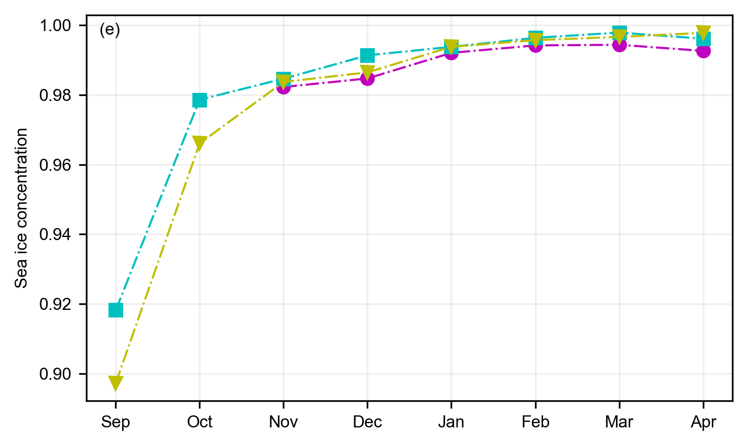
static_winter_comparison_lineplot(book_ds_innerArctic.sea_ice_conc, years=years, start_month="Sep", figsize=(5,3), annotation='(e)', set_ylabel='Sea ice concentration', save_label=save_label, legend=False)
static_winter_comparison_lineplot(book_ds_innerArctic.ice_type, years=years, start_month="Sep", figsize=(5,3), annotation='(f)',set_ylabel='Multi-year ice fraction', save_label=save_label, legend=False)
Let’s take things a bit further and set some conditions on the plots. Storing our data in an xarray dataset makes this very easy!
# Produce timeseries just using grid-cells of multi-year ice type (ice_type =1)
#static_winter_comparison_lineplot(out, title="Multiyear ice", years=years, figsize=(5,3), start_month="Nov", set_ylabel='Sea ice thickness (m)', save_label=save_label, legend=True)
# Produce timeseries just using grid-cells of first-year ice type (ice_type = 0)
# Use the flag at the start of this section to generate all plots based o the ice type classification
#out = book_ds_innerArctic.ice_thickness.where(book_ds_innerArctic.ice_type==0)
#static_winter_comparison_lineplot(out, years=years, figsize=(5,3), title="First-year ice", start_month="Nov", set_ylabel='Sea ice thickness (m)', save_label=save_label, legend=False)
Play around with some other conditions and see how things look!